The usahex maps do not need a coordinate reference system (CRS) because they are not based on actual latitude/longitude coordinates.
This is different from the hex map available from R Graph Gallery; Data for this hex map can be downloaded as a geojson file here. Since this is a geojson file; a CRS is required in order to square the a hexagons.
The differences are illustrated below.
sf_usahex <- get_coordinates("usa51")
sf_latlong <- read_sf("us_states_hexgrid.geojson") |>
  # rename abbreviation to match usahex variable name
  rename(abbr_usps = iso3166_2) |>
  # join to add other abbreviations and fips
  full_join(st_drop_geometry(sf_usahex), by = "abbr_usps")
gg1 <- ggplot(sf_latlong) +
  geom_sf() +
  labs(title = "latlong - hexagons vary in size") +
  theme_void()

gg2 <- ggplot(sf_usahex) +
  geom_sf() +
  labs(title = "usahex - all hexagons are the same size") +
  theme_void()

plot_grid(gg1, gg2)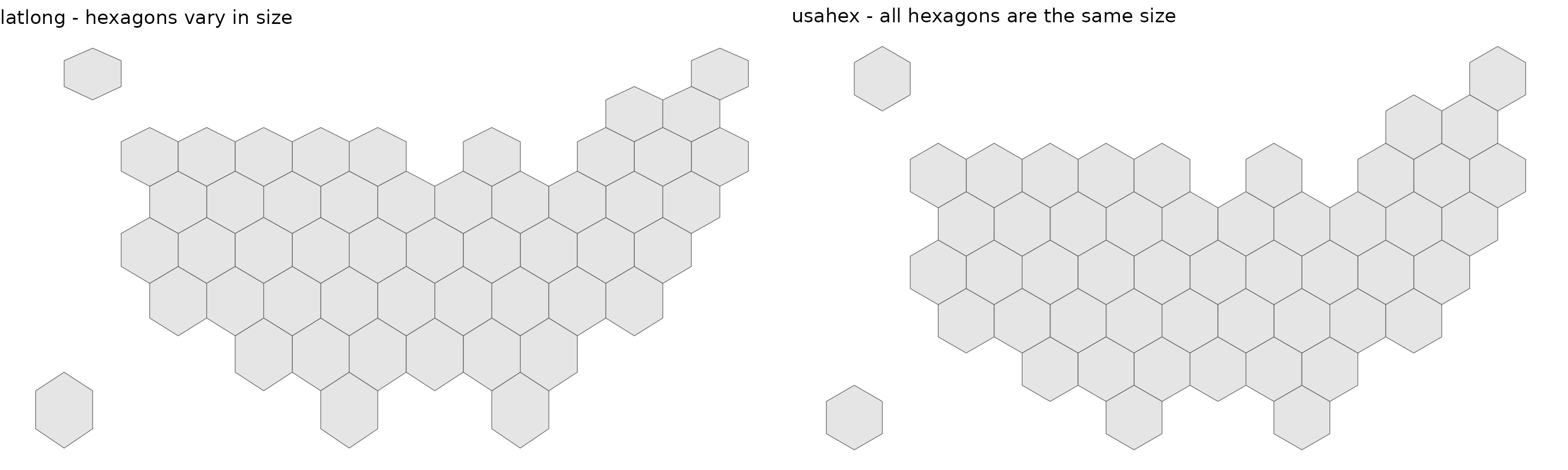
The map with hexagon’s based on actual lat/long coordinates results in the hexagons looking slightly ‘warped’ when plotted in ggplot; the hexagons at the top of the map look smaller than the hexagons at the bottom of the map. usahex hex map is not based on lat/long coordinates. All hexagons are the same size when plotted.
In order to ‘square’ the hexagons based on lat/long coordinates, you need to update the CRS.
Again, usahex coordinates are not based on lat/long, a CRS is not required for plotting.
Update CRS to Square Hexagons
It’s possible to ‘square’ the other hex map by changing the coordinate reference system (CRS) to the WGS 84 / Pseudo-Mercator CRS (EPSG code 3857).
sf_latlong <- st_transform(sf_latlong, 3857)
gg1 <- ggplot(sf_latlong) +
  geom_sf() +
  geom_sf_text(aes(label=abbr_usps)) +
  labs(title = "latlong - hexagons look the same size when change CRS to 3857") +
  theme_void()

gg2 <- ggplot(sf_usahex) +
  geom_sf() +
  geom_sf_text(aes(label=abbr_usps)) +
  labs(title = "usahex - all hexagons are the same size without CRS") +
  theme_void()

plot_grid(gg1, gg2, nrow = 1)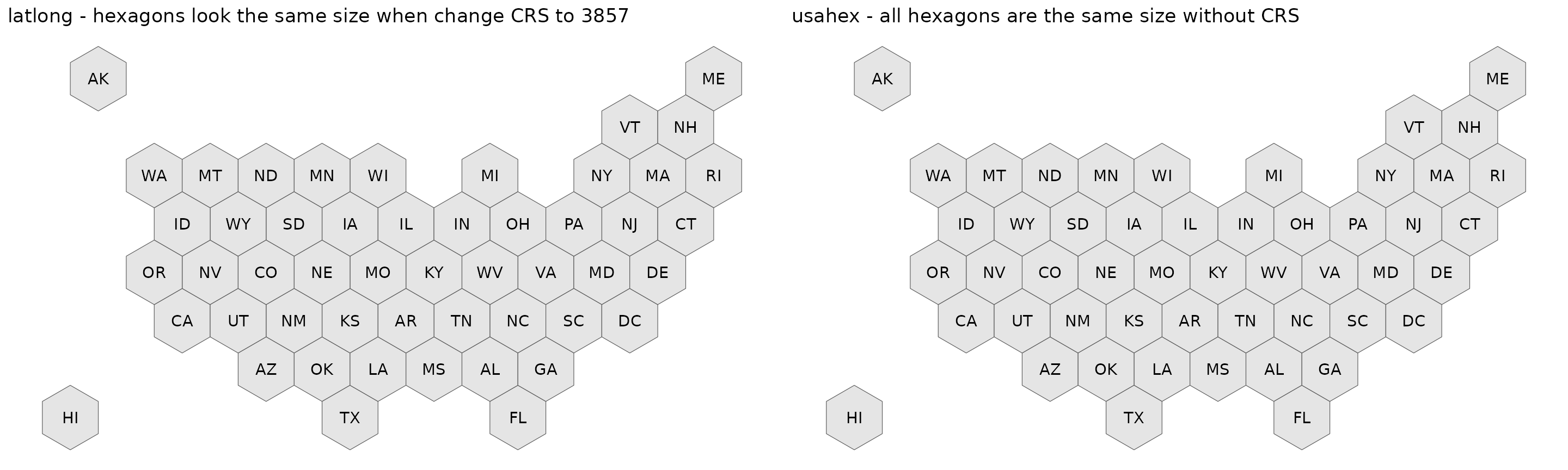
Two Labels for Each State
In order to plot two different labels, you will need to have two different points. Both the latlong hex map and the usahex map will need to be transformed. The latlong needs large numbers in order to adjust the plot location (+/- 100000) becuase the coordinates are actual lat/long values. The usahex maps only needs a small +/- 5 units to adjust the labels.
gg1 <-ggplot(sf_latlong) +
  geom_sf() +
  geom_sf_text(
    data = mutate(sf_latlong, geometry = geometry + c(0, 100000)) |>
      sf::st_set_crs(3857),
    aes(label=abbr_usps),
    fontface = "bold",
    size = 3.25
  ) +
  geom_sf_text(
    data = mutate(sf_latlong, geometry = geometry + c(0, -100000)) |>
      sf::st_set_crs(3857),
    aes(label=fips),
    size = 2.25
  ) +
  labs(title = "latlong -large adjustment values") +
  theme_void()

gg2 <- ggplot(sf_usahex) +
  geom_sf() +
    geom_sf_text(
    data = mutate(sf_usahex, geometry = geometry + c(0, 5)),
    aes(label=abbr_usps),
    fontface = "bold",
    size = 3.25
  ) +
  geom_sf_text(
    data = mutate(sf_usahex, geometry = geometry + c(0, -5)),
    aes(label=fips),
    size = 2.25
  ) +
  labs(title = "usahex - small adjustment values") +
  theme_void()

plot_grid(gg1, gg2, nrow = 1)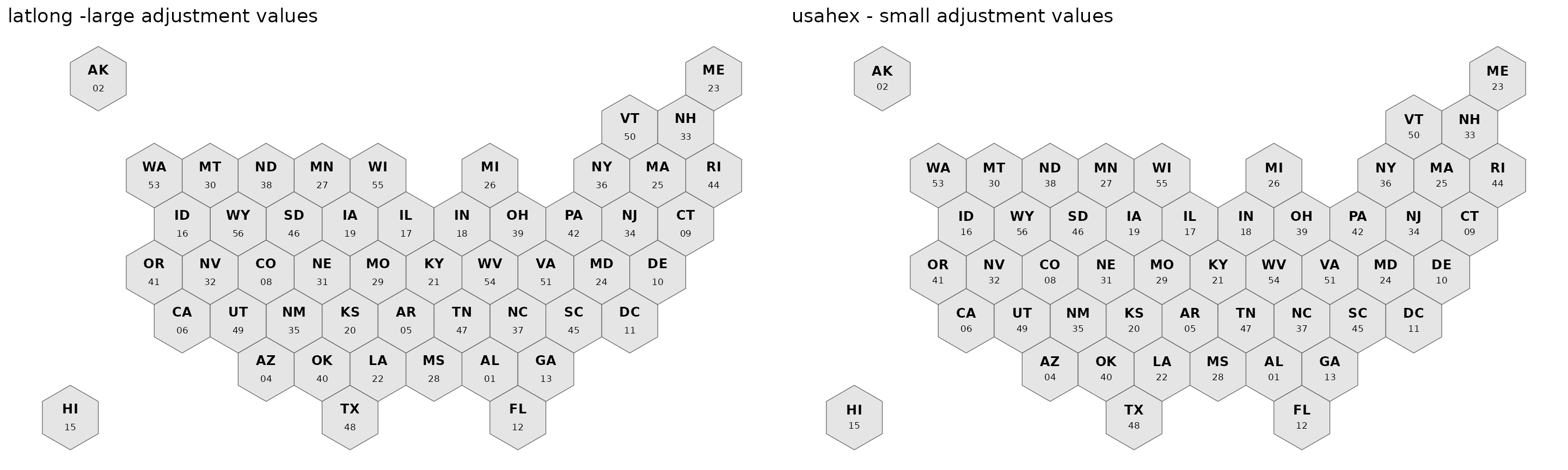
usahex geogjson files and CRS
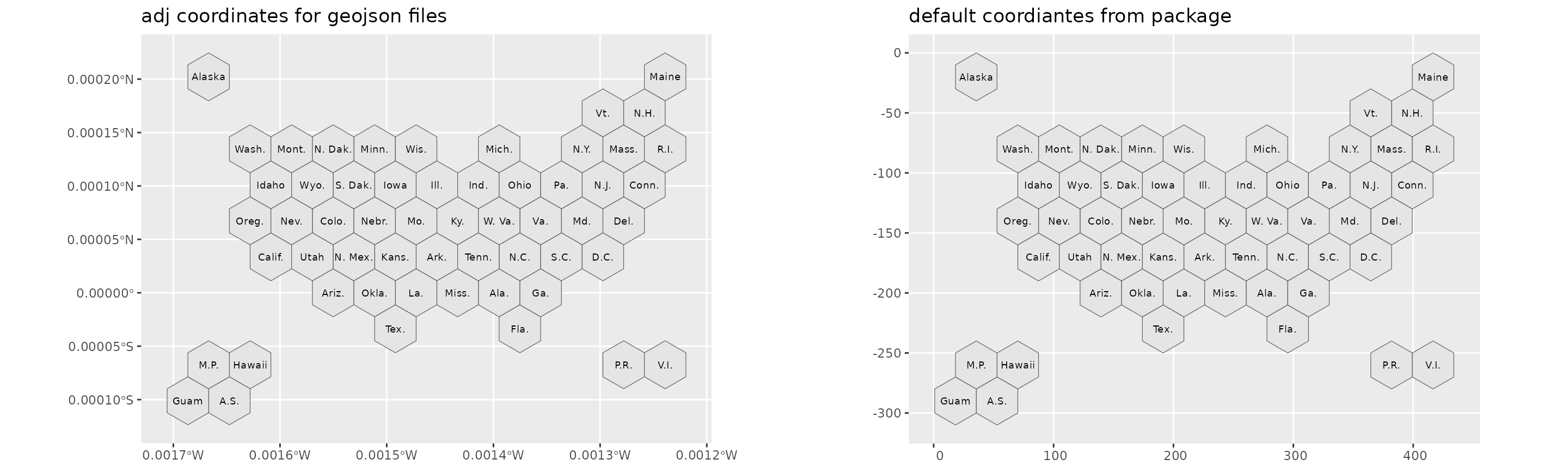
Although the R package data does not require a CRS, the geojson data avialable on github does have a CRS. In order to have the geojson files ‘play nice’ I needed to make updated to the coordinates.
The original coordinates do not fit onto a map as many hexagon values fall outside the lat/long boundaries. I adjusted the coordinates to make the hex map smaller and the shifted the map to be in the middle of the pacific ocean (based on lat/long coordinates). Finally I added the common CRS of WGS 84 / Pseudo-Mercator (EPSG code 3857).
I’m hoping these adjustments will make the geojson files easy to plot.
You can view the difference in coordinates easily by reviewing any state:
link <- "https://raw.githubusercontent.com/MarEichler/usahex/refs/heads/main/data-raw/geojson/usa56.geojson"
usa56_gj <- sf::read_sf(link)
usa56 <- get_coordinates("usa56")

filter(usa56_gj, abbr_usps == "AL") |> pull(geometry)
#> Geometry set for 1 feature
#> Geometry type: POLYGON
#> Dimension:     XY
#> Bounding box:  xmin: -157.4135 ymin: -2.5 xmax: -153.0833 ymax: 2.5
#> Projected CRS: WGS 84 / Pseudo-Mercator
#> POLYGON ((-155.2484 2.5, -153.0833 1.25, -153.0...
filter(usa56,    abbr_usps == "AL") |> pull(geometry)
#> Geometry set for 1 feature
#> Geometry type: POLYGON
#> Dimension:     XY
#> Bounding box:  xmin: 260.6922 ymin: -220 xmax: 295.3332 ymax: -180
#> CRS:           NA
#> POLYGON ((278.0127 -180, 295.3332 -190, 295.333...
The output of either file will look the same (evenly sized hexagons), but they will be on different coordinates:
gg_gj <- ggplot(usa56_gj) +
  geom_sf() +
  geom_sf_text(aes(label = abbr_gpo), size = 2.5) +
  labs(title = "adj coordinates for geojson files", x = NULL, y = NULL)

gg_pkg <- ggplot(usa56) +
  geom_sf() +
  geom_sf_text(aes(label = abbr_gpo), size = 2.5) +
  labs(title = "default coordiantes from package", x = NULL, y = NULL)

plot_grid(gg_gj, gg_pkg, nrow = 1)